Available with Image Server
The Distance Accumulation and Distance Allocation tools replace the legacy cost distance tools. These new tools measure cost distance in all directions by reconstructing a continuous accumulative surface instead of finding paths through a network of cell centers You can create output accumulative cost surfaces from input cost friction surfaces and other parameters. As with other surfaces, you can gain more precise understanding of the results by adding contour lines (lines of equal accumulative cost), visualizing them in 3D, and visualizing them in combination with allocation watersheds. Typically, the goal of constructing this surface is to plot least cost paths, which are paths of steepest descent.
Accumulative cost surface
The algorithm used by these tools reconstructs a surface from its slope.
Surface reconstruction approach
With the Distance Accumulation and Distance Allocation tools, finding least accumulative cost is no longer a network problem. The output accumulative cost raster is a surface with a shape that is unknown. You want to discover the shape given only its slope at each cell in the study area. This approach uses concepts from differential geometry to calculate true distance and costs in all directions.
The accumulative cost surface answers three important questions:
- Where does cost increase rapidly as a function of distance?
- Which source cells are closest to a given nonsource cell?
- Which path should be followed from a nonsource cell to the closest source cell?
You can use 3D views and contour lines with the output surface to find the answers to these questions. You can use the Distance Allocation and Optimal Path as Line tools to get more precise answers.
The subsections below describe the relationship between a simple input cost friction surface and the output accumulative cost surface.
Simple input cost friction surface
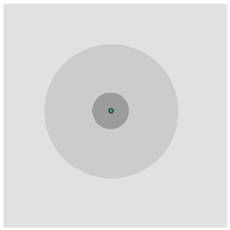
Consider a simple cost friction raster that has a central section with cost = 3, a middle section with cost = 2, and an outer section with cost = 1.
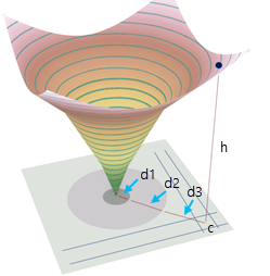
The 3D interpretation can be used to understand the relationship between the cost friction raster and the output accumulative cost surface. The height h of the surface at cell c is the sum of the slopes from the input cost raster multiplied by the distances over which those slopes are active (h = 3 * d1 + 2 * d2 + 1 * d3).
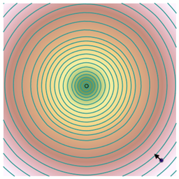
A plan view of the same output surface shows how contour lines depict accumulative cost change. The slope and aspect values at the cell location c are also shown. Aspect (the direction of steepest descent) is always at right angles to the contour line.
Incorporate least accumulative cost
A slightly more complicated case is shown below. The accumulative cost (elevation) at a nonsource cell will come from the source that arrives at that cell with the least cost.
The cost raster has two values: 1 as light gray and 3 as dark gray. The sources points are S1 and S2. Nonsource cell D is closer to S1 in terms of accumulative cost.
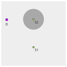
Adding contour lines to the accumulative cost surface can help you visualize how quickly cost changes as you move away from sources. By starting at the nonsource location and moving at right angles to contour lines, you travel back to the closest source cell. The path does not go to the geometrically closest source because of the high cost around that source.
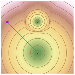
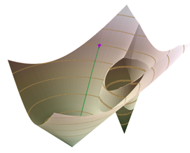
A 3D view showing the same least accumulative cost surface is below. The surface is much steeper around the expensive source (cost accumulates more rapidly). That source owns the minimum cost surface only very close to it. In all other cells in the study area, the surface is owned by the source on the left.
Allocation regions as watersheds
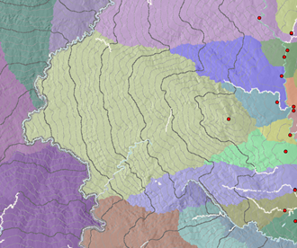
As the input cost friction surface and output accumulative cost surface become more complicated, you can still use contour lines, slope, and aspect to understand the behavior of the accumulative cost surfaces. In addition, the allocation regions around sources function as watersheds on the accumulative cost output surface. All least cost paths within an allocation region flow to the same source. Allocation watersheds are combined with contour lines and a 3D view in the examples below.
More complicated accumulative cost surfaces, such as this travel time surface, can be visualized precisely in 2D and 3D using contour lines (isochrones in this case).
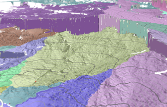
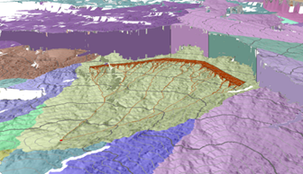
A 3D view of the same surface is shown in the following image. The cliffs in the background are barriers caused by the presence of a river.
Least cost paths flow down the accumulative cost surface toward the source that defines the allocation zone (watershed), as shown in the following image:
Surface reconstruction algorithm is an extension of the network algorithm
To find an accumulative cost surface using only knowledge of the steepest slope value at each cell, you can also use the surface reconstruction algorithm. This algorithm is similar to the shortest path algorithm used by the legacy cost distance tools but with an extra step to provide an accumulative cost approximation that doesn’t follow one of the eight network directions. This is called the Eikonal step. A brief description follows and more details can be found in Sethian, 1999.
To understand this step in context, you’ll find the accumulative cost z5 for the center cell below. Assume that you know all of the neighbor accumulative costs zi. Also, from the input cost raster, you know the slope value S at the center cell.
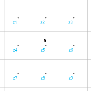
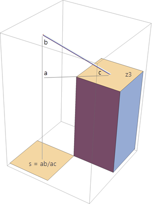
For example, one approximation for z5 can be along the diagonal between z3 and z5, where z5 = z3 + 1.4 * cellsize * S, as shown in the figure below. In this case, S—the value from the input cost raster—is interpreted as the slope of the triangle abc. For all such network style approximation, only the slope at z5 is used to approximate the accumulative cost at z5. This is different than the legacy network algorithm, which uses an average of costs from pairs of cells.
Eight network approximations can be made including four that use pairs of existing heights, as shown in the sequence of three figures below. In this case, the value of the input cost raster at the location of cell z5 is interpreted as the magnitude S of the gradient of the plane passing through the two known points and the unknown elevation z5. From this relationship, you can solve for z5. This is the Eikonal step.
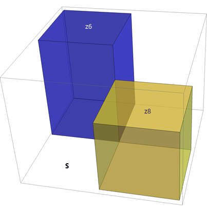
The magnitude of the gradient of the plane is calculated.
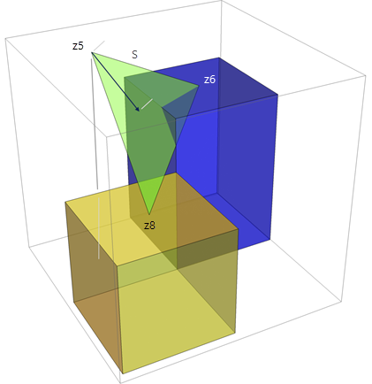
The direction of the gradient is calculated.
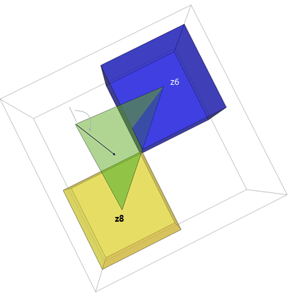
The Eikonal step also recovers the aspect information at z5, which is called the back direction.
There are now twelve approximations for the elevation at the center cell. The minimum of them is selected and recorded as the accumulative cost value z5 for the center cell. If you requested a back direction raster, the aspect of the gradient (as described in the previous paragraph) is recorded at the corresponding location in the output back direction raster.
This process is repeated for a cell every time a new elevation value for one of its neighbors is obtained. Eventually, the elevation values stop changing and the algorithm terminates. The initial elevations are supplied by the sources: they are either zero or the per-source initial accumulation value. The other initial elevation values are set to infinity. The details are described in Sethian (1999). The Esri implementation of this is a combination of techniques described in Sethian (1999) and Zhao (2004).
In summary, starting from each cell’s slope, these steps reconstruct both the elevation of the accumulative cost surface and the direction of steepest descent.
Least cost paths
Least cost paths follow the steepest downhill direction over the accumulative cost surface. That direction, for one cell, is shown above in figure 8. The output back direction raster stores that direction for each cell. You can use the Optimal Path As Line tool, with the back direction raster as an input, to plot those paths starting from any nonsource cell.
In the figures below, a curved least cost path is shown starting from the blue nonsource cell d in the upper right and travelling to the lower source cell s. While d is geometrically closer to the top source, due to the high cost around that source, it is cheaper to travel to s following the curved path.
The destination d is the blue square. It travels through an area of lower cost to the source that it can reach most cheaply, curving around the high cost source to do so.
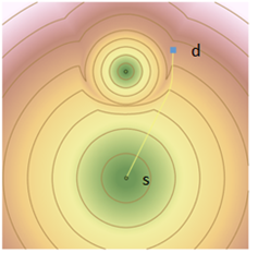
While it may appear that the name is counterintuitive, the input locations for least cost path construction are referred to as destinations. The sources were used to construct the surface and are the locations where the least cost paths terminate.
The allocation zones around the sources further clarify that the least cost path from the destination will travel to the bottom source and not the top source. Next, the selected area will be zoomed in on to show how the cell values in the back direction raster are interpreted.
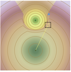
The lattice connecting back direction cell centers is shown in dark gray. The cell boundaries are shown in light gray and the cell values are shown as azimuth arrows. As the least cost path crosses lattice lines, it uses the azimuth in the closest back direction cell in the direction of travel to update its direction. At the top path vertex next to cell a, the back direction value stored in a will be used to direct the line leaving that vertex. The next lattice line to be crossed is closest to cell b, so that azimuth will be used to exit the second vertex, and so on.
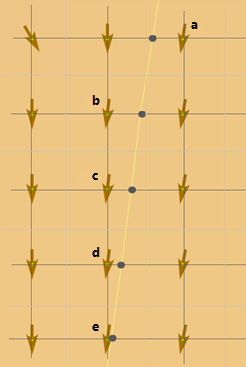
In summary, least cost paths start and end at cell centers. Other path vertices can be anywhere on the lattice of horizontal and vertical lines running through the cell centers.
Effective slope calculation
The slope values described in the previous section do not strictly come from the input cost friction raster. There are several other inputs which, together, determine the effective slope used by the surface reconstruction algorithm. A detailed description of these inputs, including the importance of accounting for direction of motion through a cell and direction of travel either from or to a source, are presented in other topics. Here, the focus is on how the inputs are used by the surface reconstruction algorithm. The inputs are the following:
- The cost friction input, C
- The surface input, S
- The source cost multiplier, M
- The horizontal factor function, HF
- The vertical factor function, VF
The effective slope used by the reconstruction algorithm has this general form:
Effective slope = C * S * M * HF * VF
This value is then multiplied by either the cell size or sqrt(2) * cell size and added to an existing height to obtain one of the network direction height estimates. A more complicated function of effective slope is used to obtain a height estimate for the Eikonal step.
The effective slope must have units of accumulative cost divided by linear distance, a rate. For example, if your accumulative cost surface is to measure travel time in hours and your analysis cell size is in meters, the effective slope must have units of hours/meter.
Since the effective slope is a product of several terms, you must ensure that the units of the individual terms combine to produce the correct effective slope units. For example, if you are using only a simple cost friction raster to describe travel time independent of direction, your cost friction raster cell values must have units of hours/meter. Alternatively, if you are also using Tobler’s hiking function as your vertical factor function, that hiking function will have units of hours/meter and your cost friction surface, if present, must be interpreted as a unitless weight. You must then ensure that your cost friction cell values can be interpreted in that way. In other words, your vertical function and cost friction cannot both be rates.
You don’t directly control surface input (S). It is a unitless weight that stretches the cell size to cover the actual 3D surface distance between cell centers. In Figure 2, the surface reconstruction algorithm calculates a height z5 for the center cell by making multiple approximations for that height using the slope from the input cost friction raster at the center cell, along with assumed known heights for the neighbor cells.
Barriers are edge connected
Barriers in the Distance Accumulation and Distance Allocation tools are input cells that cannot be passed through. They are represented as NoData cells during the computation. They are presented either explicitly as a tool parameter or implicitly as NoData values in one of the other raster inputs (such as the cost friction raster). In the first case, they are rasterized and turned into NoData in the cost raster. Since the surface reconstruction algorithm cannot lower the height estimate for a barrier cell, it will find a way around it instead.
The surface reconstruction algorithm uses all eight neighbors of a cell to find its height estimate. Corner-connected barrier neighbors will not prevent a diagonal neighbor from being used to obtain a height estimate. In the image below, a height estimate for z5 can be obtained from z3, even if cells z2 and z6 are barriers.
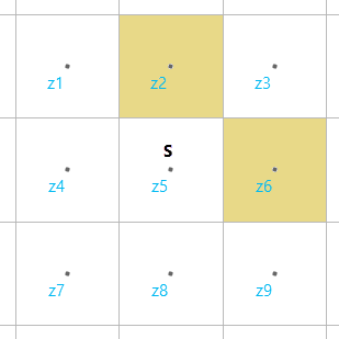
If z2 and z6 were intended to be part of a linear barrier feature, such as a canal or river, this behavior would defeat the intent of the barrier. To prevent this, the surface reconstruction algorithm favors connecting barrier cells over connecting nonbarrier cells. This means that additional NoData cells are introduced into the cost raster to ensure that all existing barriers cells share an edge. In the image above, either cell z5 or cell z3 would also become a barrier cell.
When using barriers in your analysis, consider this behavior and adjust the analysis cell size accordingly so that intended connectivity around barriers is preserved. You can use the Focal Statistics tool to thicken raster versions of linear features to use them either as barriers or as linear networks, which should not be interrupted by adjacent barrier cells.
References
Douglas, D. "Least-cost Path in GIS Using an Accumulated Cost Surface and Slopelines", Cartographica: The International Journal for Geographic Information and Geovisualization, 1994, Vol. 31, No. 3, DOI: 10.3138/D327-0323-2JUT-016M
Goodchild, M.F. "An evaluation of lattice solutions to the problem of corridor location", Environment and Planning A: Economy and Space, 1977, vol. 9, pages 727-738
Sethian, J.A. Level Set Methods and Fast Marching Methods (Evolving Interfaces in Computational Geometry, Fluid Mechanics, Computer Vision, and Materials Science) 2nd Edition, Cambridge University Press, 2nd edition (June 1, 1999)
Warntz, W. "Transportation, Social Physics, and the Law Of Refraction", The Professional Geographer, 1957, Vol. 9, No. 4, pp. 2-7.
Zhao, H. "A fast sweeping method for Eikonal equations", Mathematics of Computation, 2004, Vol. 74, No. 250, pages 603-627