Available with Image Server
Once the straight-line distance is calculated and possibly adjusted for barriers and a surface raster, the rate that distance is encountered can be determined. The cost surface is one of four factors that affect the rate at which the distance is encountered. The other three are source characteristics, vertical factor, and horizontal factor.
The cost surface captures what the traveler encounters as they move through the landscape. Travelling across a field is easier than moving through a forest, which is easier than moving through a swamp. Each value in the cost surface is multiplied by the adjusted straight-line distance to determine the rate the distance is encountered by the traveler.
As a result of the cost surface, the traveler can cover the adjusted straight-line distance units at a faster rate in a field than in a forest or a swamp.
Straight-line distance is in linear units such as meters or feet. When determining the rate the distance is encountered, the units can be dollars, preference, energy expended, or risk. The rate is a cost per unit of distance measurement.

Creating a cost surface is a multistep process. First identify the criteria that will affect the movement. Then transform the criterion values to a common cost scale. Finally, weight and combine the criteria.
This type of analysis is known as least-cost analysis. A cost surface is also referred to as an impedance or friction surface. It is more difficult, expensive, or slower to cover the adjusted straight-line distance units in high cost locations. Creating a cost surface can be similar to creating a suitability surface; however, in a suitability surface, the higher values are preferred. In a cost surface, the lower values are easier to move through.
Various factors can be combined to create the cost surface. For example, when creating a cost surface for animal movement, factors such as land-use type, distance from roads, and distance from water are used to capture the preference of the animals as they move through the landscape. Because the values in the criteria have different meaning, each of the criteria must be transformed to the same cost scale before they are combined.
In many cases, the cost surface defines the cost units for the cost distance analysis. The source characteristics, the vertical factor, and the horizontal factor are multipliers of those units. Each multiplier should be relative to the same cost units defined in the cost surface. If more than one of the four rate controlling factors (cost surface, source characteristic, vertical factor, and horizontal factor) are specified, only one of them can have units, with the other factors being unitless multipliers modifying those units.
The cost surface allows you to simulate the traveler on an actual landscape.
Cost surface use examples
A cost surface can be used to solve various scenarios, such as the following:
- Identify the cheapest route to construct a road to a proposed school. The cost surface units are dollars per meter for construction.
- Connect the wildlife habitat patches with corridors to allow the species to move between the patches. The cost surface units are preference per foot for movement through the features at each location.
- Locate a new pipeline to connect petroleum fields to a refinery. The cost surface units are based on the environmental impact the pipeline will have on each location.
- Determine the fastest way to reach an injured hiker in a remote area. The cost surface units are minutes per meter.
Incorporate a cost surface
Distance analysis can be divided conceptually into the following related functional areas:
- Calculate straight-line distance and optionally adjust the calculations with a barrier or surface raster.
- Once the straight-line distance is calculated, optionally determine the rate the distance will be encountered through a cost surface, source characteristics, vertical factor, and horizontal factor. Create the accumulative distance raster.
- Connect regions over the resulting accumulative distance surface using an optimal network, specific paths, or a corridor.
From the second functional area, determining the rate the distance will be encountered through a cost surface is illustrated below. The scenario involves a collection of four forest ranger stations (purple dots), and some rivers (blue lines).
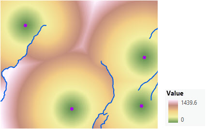
Adding a cost surface simulates a traveler moving through the landscape. Notice in the image below the distances do no radiate evenly from each of the stations.
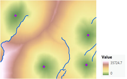
Cost surface for rate of straight-line distance
To create a cost surface for determining the rate the adjusted straight-line distance will be encountered, you'll do the following:
- Identify the criteria to define the factors that affect the movement. These criteria will capture how the traveler will encounter the distance as they move through the landscape.
- Some data, such as land use, can be used directly as criteria. Other criteria—such as aspect, distance from a feature, or visibility—must be derived from the base data. The spatial analysis tools that can be used to create these derived criteria include Distance Accumulation, Aspect, Geodesic Viewshed, Calculate Density, and Surface Parameters.
- Transform the criteria to a common scale. This can be done with the Remap tool.
- Weight and combine the transformed criteria. Use the Weighted Sum tool for this.
Cost surface affects the rate distance is encountered
A cost surface identifies the cost, impedance, friction, or preference of each location relative to movement based on the features at the locations. Regardless of the potential application, or the cost units being modeled, the general workflow is similar.
Absolute costs such as cost of construction, time, or energetics are ideal, but they can be difficult to define for each location. However, for many applications, no single absolute cost units exist. For example, if you are creating a cost surface to identify a hiking or biking trail between two locations, using energy or time for cost units alone will not capture other factors that influence where the trails should go. Those factors can include scenic views, land ownership, and avoiding environmentally sensitive areas. When creating a cost surface for creating wildlife corridors, the animal may balance between moving within good habitat with being safe. In both cases, there is no single cost unit that can capture the scope of the movement decisions.
In these cases, relative subjective cost units such as preference, security, and risk are used. Each of the criteria values is assigned to a common cost scale with the assigned costs being relative to each other based on the subjective units. That is, a cost of 10 is twice as difficult to move through than a cost of 5. Each value in each criterion is placed on the same common cost scale.
If the cost surface is defining the units for the cost analysis, the other rate controlling factors—source characteristics, vertical factor, and horizontal factor—are unitless multipliers modifying the specified cost units.
Absolute cost units can be directly assigned using any number of Spatial Analyst tools. When defining the subjective cost units to create the cost surface, the workflow described below is often used.
Cost surface workflow
The workflow for creating a cost surface when specifying relative costs is as follows:
- Identify criteria that affect the cost of movement and gather base data.
- Derive criteria from base data as necessary.
- Transform the values of each criterion to a common cost scale.
- Weight criteria relative to one another and combine them to create a cost surface.
Once the cost surface is created, you can connect regions with the least-cost paths over that cost surface.
As was previously mentioned, creating a cost surface follows similar steps to creating a suitability surface. The common steps between them are identify the criteria, gather the base data, derive necessary criteria from the base data, transform the criterion values to a common scale, weight the criteria, and combine the criteria. Unlike in the final suitability surface in which higher values are preferred, in the cost surface, the lower values are preferred for movement because they represent lower costs. The cost surface is used for least-cost analysis. As a result, when implementing the transformations, the more preferred locations for movement receive lower values.
In the following sections, an example application of this workflow is described. The goal is to identify wildlife corridors for bobcats to move between habitat patches. The workflow is for demonstration purposes only and does not realistically define all bobcat interactions. The workflow described above can be applied to create cost surfaces for many other applications.
Define the goal and cost units
First, define the goal of the movement. The goal will vary depending on the problem being solved. For example, the goal for a cost surface to be used to locate a powerline may be to minimize the cost to construct it. When locating a route for firefighters to move resources between two fires, the goal may be to move between the fires as quickly as possible. For the bobcat scenario, the goal of the cost surface is to allow the bobcats to move safely between the habitat patches while at the same time maintain access to certain resources.
Next, the units of cost must be established. For siting the power line, each criterion can be transformed based on the cost for construction. For locating the firefighting route, the cost units may be time. For the bobcat corridors, defining the units presents two challenges. One is that there is no objective measurable cost units. The other is that the criteria have varying objectives. For example, the distance to streams criterion is the need for water, while distance from roads is to remain safe. In this situation, the criteria must be transformed on a relative subjective preference cost scale before they can be combined.
Once the goal and units are defined, the methods for evaluating the results of the model must be established. In the bobcat cost surface, to determine if the resulting paths are successful, you could go to the corridors and see if the bobcats are using the paths to move between the patches.
The following image illustrates the creation of the bobcat cost surface:
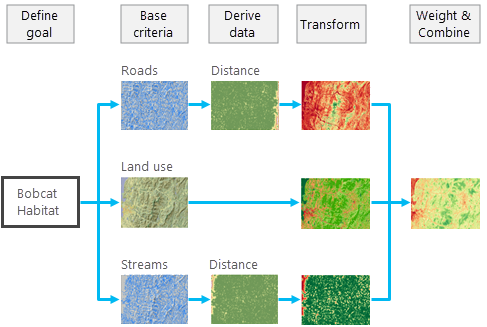
Identify the criteria that affect the cost for movement
Now that you have defined the goal, units, and evaluation methods for the analysis, the first step in creating a cost surface is to identify the criteria defining the movement. In this sample case, the criteria are the things the bobcats prefer as they move through the landscape. Each criterion identified should be instrumental in reaching the overall goal of the model, which is to ensure the bobcats can safely move between the habitat patches while accessing critical resources. The identified criteria should capture the interactions of the bobcats relative to their movement needs.
In the simplified bobcat example, the following criteria will be considered:
- Land-use types—Bobcats prefer to move through forests for cover and do not like to move in developed or semideveloped areas.
- Distance to roads—For safety, bobcats prefer to move in areas farther from roads.
- Distance from streams—For their water needs, bobcats like to stay near water sources as they move through the landscape.
Derive criteria from base data as necessary
Some criteria, such as land-use types in the bobcat example, can be used directly in the creation of the cost surface. Bobcats directly respond to the different land-use types. Other criteria must be derived. Keep in mind that it is not the roads or the streams themselves that are the criteria, rather it is the distance from the roads or the streams that the bobcats are responding to.
Since datasets for distance to roads and steams are not initially available, the appropriate tools can be used to derive these criteria from base data. Use the Distance Accumulation tool to determine how far each location is from the closest road for the road criterion and use it again to determine the distances from streams for the streams criterion.
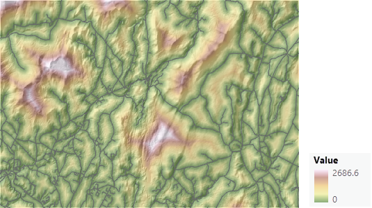
Transform the values of each criterion to a common cost scale
Mathematically adding the land use, distance to roads, and distance from streams rasters together will result in meaningless values. For example, a particular location may have a land use value of 4, representing single family residential. It is also 627 meters from a road and 2,252 meters from a stream. Adding these values together results in 2,883, an irrelevant number. Before the criteria rasters can be added together, the values in each criterion must be transformed to a common cost preference scale.
In this example, a 1-to-10 common cost scale will be used. For each value in a criterion, locations with features that are easiest or most preferred to move through will receive low cost values, and more difficult or less preferred locations will receive higher cost values. For example, locations within 100 meters of a road are least preferred and will receive a cost of 10, distances between 100 to 300 meters may be assigned a cost value of 5, and distances that are greater than 300 meters may receive a cost of 1 since bobcats prefer to travel far from roads.
When transforming the values in each criterion to the 1-to-10 cost scale, transform the values relative to one another within the scale. That is, a location assigned a cost value of 3 is twice as preferred to travel through as a location assigned a cost value of 6, and a cost value of 10 is 10 times more difficult to travel through than a location assigned a cost value of 1.
This transformation process is applied to each value in each criterion identified for the cost surface. For the bobcat model, for the land-use criterion, preferred land-use types such as forest will be assigned a cost value of 1 (preferred and less costly to move through), residential will be assigned a cost value of 5, and industry will be assigned a cost of 9. For the distance from roads criterion, locations closer to the roads will receive higher costs of 9 and 10, while locations farther away from roads will receive lower cost values (because bobcats prefer to move through them). For the distance to streams criterion, it is more preferred to move closer to the streams, so near locations will receive lower costs of 1 or 2 and distant locations will receive higher costs of 9 or 10.
It is desirable that the assigned costs have the same preference between criteria. That is, a transformed distance from roads that is assigned a cost of 5 has the same preference as a land-use type or distance to streams location also assigned a cost of 5.
To transform the criteria, a reclassification is done. The same cost scale is specified in these tools for each criterion. For this example, a 1-to-10 cost preference scale will be used.
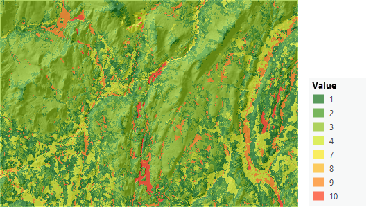
Land-use type is categorical data and a one-to-one transformation is used to map land-use types to the costs. The Reclassify tool will be used. Forest is assigned a 1 and industrial is assigned a 9, and so forth in the reclassify table.
| Value | New |
|---|---|
Agriculture | 2 |
Bare Land | 1 |
Developed, High Intensity | 9 |
Developed, Low Intensity | 5 |
Developed, Medium Intensity | 8 |
Forest, Coniferous | 1 |
Forest, Deciduous | 2 |
Forest, Mixed Deciduous-Coniferous | 2 |
Grassland | 4 |
Scrub/Shrub | 3 |
Water | 10 |
Wetland | 9 |
NODATA | NODATA |
Below is the resulting transformed land use map. Green locations are more preferred to move through and red less.
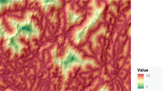
Distance from roads and distance from streams are continuous data. To transform the criteria values to capture the cost interaction, a function will be applied. With each step the bobcats take from a road, their preference or cost continuously decreases based on the specified function.
The focus of the Rescale by Function tool is for suitability modeling in which the more preferred attributes receive the higher values. In least-cost analysis, the logic is reverse. The more preferred areas to travel within are assigned low values indicating lower cost. The Rescale by Function tool can accommodate this reversal in logic in one of the following two ways:
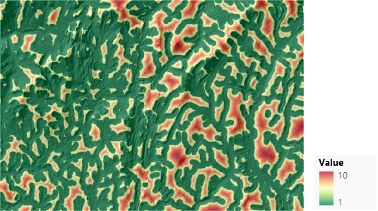
- Select the inverse of the suitability function in the tool. That is, the Small function can be applied for the distance to streams criteria in a suitability model indicating that being closer to streams is more suitable, thus receiving higher values. When distance from streams is used for the cost surface, the Large function is used, indicating that farther locations receive the higher values (less preferred). The closer locations receive the lower values (the lower costs) and are more preferred to travel through.
- The same logic used in the suitability model can be applied but in reverse. The Small function can be specified for the distance from streams criterion for the suitability model and when transforming the distance from the streams criterion for the cost surface. However, for the cost surface, the From scale and To scale parameters must be reversed from 1 to 10 to 10 to 1. As a result, the closer locations now receive the To scale value, which is now 1 since it is least costly to move through.
To capture the preference that the bobcat want to move near streams, a different function was applied to the distance from streams criterion.
If you are using absolute cost units when transforming the criteria values to the cost, such as cost of construction or time, you can use direct assignment or mathematical formulas. These formulas can be applied using the Raster Calculator instead of applying the relative transformation steps above.
Tip:
Cost values must always be positive; the input cost raster cannot have cell values less than or equal to 0. If such values exist, you can rescale the entire range to be greater than 0 or replace the problem values with small positive numbers. You can do this using the Con tool. If areas with a value of 0 represent areas that should be excluded from the analysis, turn these values to NoData before running Distance Accumulation. You can do this using the Set Null tool.
Now the values in each criterion are transformed relative to one another to a common cost scale, and the transformed criteria can be combined.
Weight criteria relative to one another and combine them to create a cost surface
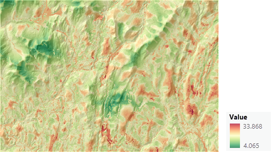
When the three transformed criteria are added together, the resulting range can be from 3 to 30. A location assigned a value of 3 is the most preferred to move through. It would be in forest, far from a road, and next to a stream. Locations assigned higher values will be less preferred (more costly to move through), based on the features located there.
However, before adding the criteria together, it may be that one criterion is more important or more significant to the movement cost for the bobcats than the others. If that is the case, that criterion will be weighted more than the others. To emphasize the distinction, the transformation process converts the values in a criterion relative to one another. The weighting defines the relative importance of each criterion to one another.
A weight is a multiplier that is applied to each transformed value in the criterion.
In the bobcat suitability model, applying a higher weight to a criterion indicates that the criterion is more important to the biology of the bobcats. In a cost surface, however, the weight indicates the criterion is more significant or costly for movement than the other criteria.
In the bobcat cost surface, it is determined, for safety, bobcats want to avoid traveling near roads. As a result, the transformed distance from roads will be assigned a higher weight than the distance from streams criterion. For example, a location may be initially assigned a cost of 10 for distance to roads since it is near a road. The location may be assigned a cost of 1 for distance to streams, since it is also close to a stream. If a weight of 1.5 is applied to the distance from roads criterion while the distance from streams criterion is assigned a weight of 1, that location will receive a total cost value of 16 (the result of 10 x 1.5 + 1) in the resulting cost surface. As a result, locations closer to roads become higher in cost and less preferred to move through.
In this example, the land use criterion will also be assigned a weight of 1.
Because of weighting, sometimes least-cost analysis is referred to as weighted least-cost analysis.
Note:
If absolute measurable cost units, such as dollars or time, are used, do not apply weights. Even though a criterion may be more or less significant, the absolute cost will not vary. The dollar cost or time are the actual costs. If a weight is applied, the absolute units are no longer valid, and the cost will then be on a relative scale.
A cost surface has now been created. Based on the features at each location, the cost surface indicates the preference of each location relative to one another for movement from the perspective of a bobcat. The final goal of the bobcat model is to connect a series of bobcat habitat areas with wildlife corridors over the resulting accumulative-cost raster, enabling bobcats to move between them.
Habit patches can be connected in the following ways:
- Create a least-cost network (see Connect regions with the optimal network).
- Connect specific patches to one another (see Connect locations with the optimal paths).
- Connect the patches using corridors (see Connect locations with corridors).
Slope and cost surface
The cost surface is one of the four factors that can control the rate at which the adjusted straight-line distance is encountered. In a cost surface, the cost is the same whether moving through the cell from east to west, west to east, north to south, south to north, or moving to and from in any diagonal direction. However, it may matter to the traveler which direction they are moving through the cell. Going uphill requires different effort than moving downhill. Thus, how that slope is encountered may matter. For example, if you move into a location that has steep slopes and you are moving perpendicular to those slopes (moving with the contour), the effort is less than it is going directly up the steep slope.
The Slope tool calculates slope by determining the rise over run from the height at the processing cell center to the heights at each of the eight neighboring cell centers. The steepest slope of the eight slopes is assigned to the cell. Since a cell is assigned the maximum descent, it does not capture any directionality of the movement into the cell. When modeling movement, it may not matter how steep the slope is at a location, but it may matter how that slope is encountered. If the slope raster is used in a cost surface, the traveler may unnecessarily avoid the cells that are assigned steep slopes.
Generally, if the direction that the traveler encounters the slopes is important, the direction needs to be captured by the vertical factor, not through the cost surface. Slope is often incorrectly used as an input criterion in a cost surface.
However, there are cases when a slope raster is appropriate to include in a cost surface. For example, you're locating a new hiking trail and the slope in a cell is so steep that regardless of the direction the traveler enters the cell, the slope slows down the traveler. In this case, the directionality of the slope does not matter so it is appropriate to include the slope raster in the cost surface.
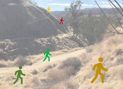
What matters to the traveler is how they encounter the slopes, not how steep it is. Going up a steep slope will require the most effort, going down the least, and moving with the slope somewhere in between. Land cover combined with the slope can also affect movement. Movement over rougher natural ground is more difficult than traveling on a road. The hikers are color coded based how easy they can overcome the encountered slopes and land cover. Green figures can travel at a faster rate than the red figures.
Units in the rate controlling factors
Once the adjusted straight-line distance is calculated, the rate those distance units are encountered is controlled by the cost surface, source characteristics, vertical factor and horizontal factor. Each factor is a multiplier to the adjusted straight-line distance. Care must be taken when specifying the units for the factors. The cost surface cannot be in preference and the vertical factor be in time. The units must be consistent.
Generally, the cost surface is the driving units for the rate analysis. The vertical factor, horizontal factor, and source characteristics are often unitless multipliers of the cost surface’s cost units.
This is not the case when applying Tobler’s hiking function using the vertical factor. In the hiking function, the units are time and become the driving units for the cost analysis. If a cost surface is added to the analysis, the cost surface values must be unitless multipliers, modifying the time to move through the landscape while accounting for the slopes in the vertical factor.
Create a cost surface using ModelBuilder
ModelBuilder is an effective environment to create a cost surface. It provides the capability to chain the input and output criteria and geoprocessing tools. The graphic representation of the model allows you to visually present the logic of the model and you can always make changes and rerun the model.
When creating complex cost surfaces that may include different movement objectives, submodels are often used. Submodels not only organize the model objectives, different transformations can be used for certain criteria to meet the different movement objectives. For instance, in our bobcat example, when transforming land-use type, it may be favorable to move near the edge of a field for the resource submodel, but unfavorable for the security submodel.
Additional cost surface applications
The following demonstrate how a cost surface can be used to address other types of applications.
No-wake zones
You can use a cost surface to represent maximum pace through a no-wake zone in a harbor. A buffer of 100 meters around the coastline may have a maximum speed of 5 knots and a maximum pace of 1h/(5*1.852)km. The buffer corridor between 100 and 200 meters may have a maximum pace of 1h/(10*1.852)km. Note that as speed increases, pace decreases.
Road construction cost
To estimate the total construction cost for a new road, you can create a cost surface that encodes per-mile construction costs. Building a new two-lane undivided road in rural areas is cheaper than building the same road in urban areas. In this case, you can classify the cells in the cost surface into urban vs. rural. Based on information in an FAQ sourced from the American Road and Transportation Builders Association (ARTBA), typical values for per-mile costs for rural cells are $2 million per mile, and $4 million per mile for urban cells. In addition, barriers can be added based on local zoning and property laws.
Additional information
The following sections contain additional information regarding cost surfaces.
Consider the time of year of the movement
The time of year may alter the cost surface. Is the cost surface for movement in the winter or summer or the dry season or wet season? Is the movement for fair or foul weather or for an extreme event or for typical conditions?
Are other temporal influences affecting the movement? For a wildlife cost analysis, is the movement for reaching calving sites, or is it for daily movement between patches or for seasonal migration? Is the movement during hunting season?
The various time factors that can affect movement may not only affect the transformations and weights; they may also influence which criteria will be used in the cost surface.
To capture the various seasonal and movement types, you may need multiple cost surfaces and to perform the distance analysis on each. You may need to combine the results to capture the full yearly movement needs.
Incorporate roads or trails into the cost surface
Consider a cost surface that will be used by rescuers on all-terrain vehicles (ATVs) to reach an injured hiker. For this example, the criteria are the land-use types, aspect, and slopes. Swampy areas will be high cost and grassy fields less costly. Since this rescue is in the spring, south facing aspects are muddier and more costly, while frozen north facing aspects are less costly. The difficulty to overcome the slopes can be incorporated through the vertical factor.
When a road is encountered, the cost changes. It is faster and easier to travel on the road. The cost to move on the road is a low constant cost.
To capture the constant low cost of the road, once the cost surface is created, the roads are burned into the cost surface.
- Rasterize the roads with the Convert Feature to Raster tool, and assign a single cost to the roads. If the roads feature dataset has no cost field, rasterize on any field with values of 0 or greater, such as FID, and apply the following expression in the Raster Calculator tool: Con(rasterRoads >= 0, 50)
50 is the assigned cost. The resulting raster will be named roadCostValue and used as input into the expression in the next step.
If applicable, the cost can vary by road type.
- Convert the NoData values to zero using the Con and IsNull tools from the list in the Raster Calculator tool. Use an expression in the form of: Con(IsNull(roadCostValue), 0, roadCostValue).
The resulting raster is named roadCost and is used as input into the expression in the next step.
- Burn in the roads into the cost surface using the Raster Calculator. Use an expression in the form of: Con(roadCost > 0, roadCost, costSurface)
In the final output raster, cells that a road passes through will be assigned the cost associated with the road. All nonroad cells will receive the cost value created in the cost surface.
As a result, the ATV will move through the landscape, and when it encounters a road, it will travel on that road as long as possible before leaving it to reach the injured hiker. The cost of the road can be further refined for steep and curvy sections.
Thicken barriers to prevent cracks
You can incorporate linear features, such as roads or rivers, that have high cost or are barriers into your cost surface. If the linear feature is a polyline, it will be rasterized. When represented as a raster, the linear feature will only be one cell thick. While the nature of the barrier would be preserved where it is perfectly horizontal or vertical, it may be diagonal. In this case, it may be geometrically possible for the traveler to slip through what amounts to cracks in the barrier. If that happens, the barrier or high cost cells are no longer a hindrance to the movement.

To add a linear feature to the cost surface, complete the following steps:
- Buffer the linear feature at least larger than the diagonal of the cell distance of the cost surface.
- Rasterize the resulting buffered feature using the Polygon to Raster tool.
- Assign all the rasterized buffered cells to the cost and assign all NoData cells to zero. Using the Raster Calculator tool, enter an expression in the form of: Con(IsNull(buffRaster), 0, 35).
The value 35 is the cost for the linear feature.
If the linear feature is a true barrier, set the buffered cells to NoData by specifying nothing for the false statement (the 35) identified in the previous expression.
- Add the resulting raster from step 3 to the cost surface as described in the previous section.
These same steps are used if the input linear feature is a raster. You do not need to first rasterize the linear raster feature. Create the buffer around the raster feature using the Distance Accumulation tool and setting a Maximum accumulation (a distance) value.
Instead of buffering the linear feature, you can rasterize the linear feature if it is not already a raster. Then run the Focal Statistics tool on the rasterized linear feature specifying the statistic. The tool will widen the linear feature by one cell on either side of the feature if a 3 by 3 neighborhood is selected. The assigned cell values will be based on the specified statistic. The resulting surface can then be added to the cost surface as described in the previous section. This approach is particularly useful if the linear feature is a raster and it represents a gradient such as depth, salinity, pH, or distance.
Note:
If a high cost is to be assigned to the linear feature in a relative cost scale, ensure that the assigned costs are relative to the summed values in the final cost surface.
However, if that linear feature is a true barrier, assign the cells NoData before they are combined in the cost surface. If the linear feature is a true barrier, it is better if it is entered through the barrier parameter in the Distance Accumulation tool.
Use the Suitability Modeler to create a cost surface
While you can create a cost surface using individual geoprocessing tools, you will need to keep track of the tools you use and the specified parameters so you can make subsequent changes. Creating a cost surface using ModelBuilder is the recommended method.
A cost surface can also be created in the Suitability Modeler. If you are using the Suitability Modeler to create a cost surface, remember that in a suitability model, the more favorable a criterion value is, the higher suitability it receives. A cost surface is used to perform least-cost analysis. The areas that are easier or less costly to move through will receive a lower value.
The Unique Categories and Range of Classes transformation methods in the Suitability Modeler are a one-to-one assignment of the cost value to the category or class. In the Continuous Functions transformation method, you need to apply the opposite function than you would in a suitability model. For example, if being closer to streams is more preferred in a suitability model, you can apply the Small transformation function. The smaller or closer locations receive the higher suitability value. If moving near streams is more preferred or less costly in a cost surface, you can select the Large function. The farther away locations will be transformed to higher values, which are more costly. The closer locations will receive the lower values, which are less costly and more preferred to travel through.
Alternatively, you can use the same logic for selecting the continuous functions as you do for suitability modeling. The more preferred locations receive the higher value, but in a cost surface the more preferred locations to move through should receive lower values. To reverse the values for the cost surface, use the Invert function parameter in the Continuous Functions method.