Available with Image Server
A barrier is an obstacle that is present between the two locations you are calculating the distance for. Barriers can be features such as a lake, a divided highway, or a mountain range. The straight-line distance is altered when a barrier exists. You may want to know the shortest possible distance between your locations after accounting for the additional distance necessary to detour around the barrier.

When a barrier is in the way, the traveler must move around it.

You can adjust straight-line distance by including barriers and incorporating the actual surface distance that is traveled. Once the adjusted straight-line distance is determined, the rate that distance is encountered can be controlled by a cost surface, source characteristics, a vertical factor, and a horizontal factor. If any of these rate factors are specified with a barrier, detouring around the barrier will be the least-cost distance between the locations.
Barrier use examples
Barriers can be used to help solve various scenarios, such as the following:
- In a wildlife study, determine the distance between two habitat patches with a lake between them.
- Determine the shortest distance for a boat to travel between two marinas when there is a peninsula between them.
- Identify a hiking trail route in an area where there is a steep drop off that you need to navigate around.
- Define the flight path an airplane should take when there is a storm between it and its destination.
Adjust straight-line distance analysis with barriers
Distance analysis can be divided conceptually into the following related functional areas:
- Calculate straight-line distance and, optionally, adjust the calculations with a barrier or surface raster.
- Optionally determine the rate the distance will be encountered using a cost surface, source characteristics, vertical factor, and horizontal factor. Create the accumulative distance raster.
- Connect regions over the resulting accumulative distance surface using an optimal network, specific paths, or a corridor.
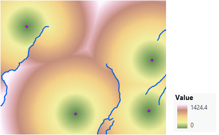
From the first functional area, the straight-line distance is adjusted with barriers as illustrated below. The scenario involves a collection of four forest ranger stations (purple dots), and some rivers (blue lines).
The straight-line distance result identifies the distance from each nonsource cell to the closest ranger station.
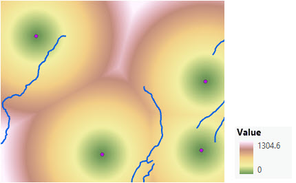
Barriers adjust the straight-line distance since the traveler needs to move around them.
The straight-line source direction and back direction rasters are the same when there are no barriers.
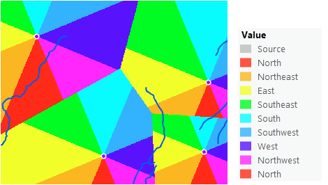
The back-direction raster identifies, for each cell, the direction to move from the cell to return to the closest source. When barriers are introduced, the traveler must move around them.
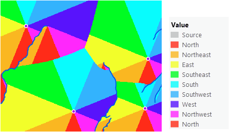
Create a distance raster with barriers
To create a distance raster that incorporates barriers, complete the following steps:
- Open the Distance Accumulation tool.
- Provide the source in the Input raster or feature source data parameter.
- Name the output distance raster.
- Identify the barrier in the Input barrier raster or feature data parameter.
- Specify any other necessary parameters.
- Click Run.
Barriers affect distance calculation
The sections below provide information about adjusting the straight-line distance with barriers using the Distance Accumulation tool.
Specify a barrier
A barrier can alter distance calculations if you need to detour around it. Examples of barriers include a lake, divided highway, mountain range, river, or cliff. There is an input parameter you can use to specify where barrier locations exist, as either feature or raster data. If the input for this parameter is a feature class, it will be converted to a raster when the tool is run.
You can define barriers in other ways, as well. If a surface raster, cost surface, vertical factor raster, or horizontal factor raster are provided, NoData cells in any of the these rasters are considered to be barriers. If the Mask environment is set, the locations that are outside the area covered by the mask—the NoData cells—are also considered to be barriers. In all cases, barriers prohibit movement. When necessary, all barriers will be thickened slightly to prevent any cracks from permitting movement through that barrier. See the Thicken barriers to prevent cracks section below to learn more.
To summarize, travel is permitted across locations that have valid values for the input surface raster, cost surface raster, vertical factor raster, and horizontal factor raster, as well as across locations that are within the mask area defined in the analysis environment if it is specified. Travel is not permitted across locations defined by the barrier input, across locations that are outside the mask area (NoData cells), or across any location where the surface raster, cost surface raster, vertical factor raster, or horizontal factor raster has a value of NoData.
Barriers affect the output distance rasters
The following output rasters produced when performing distance analysis are affected by barriers:
- Distance accumulation raster
- Back-direction raster
- Source direction raster
Distance accumulation raster
For each nonsource cell, the output distance accumulation raster calculates the accumulative distance to the closest or least-cost source. If a barrier input has been specified, the distance values account for detouring around the barrier cells.
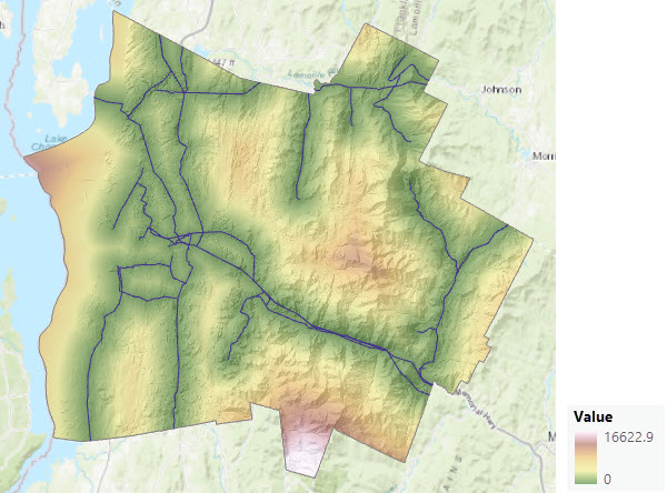
An example is locating a new building complex where proximity to existing power lines is preferable. In the following image, the distance from each nonsource cell to the closest power line (blue lines) is displayed. No barrier input was specified. The resulting distance raster is displayed, with green indicating closer locations.
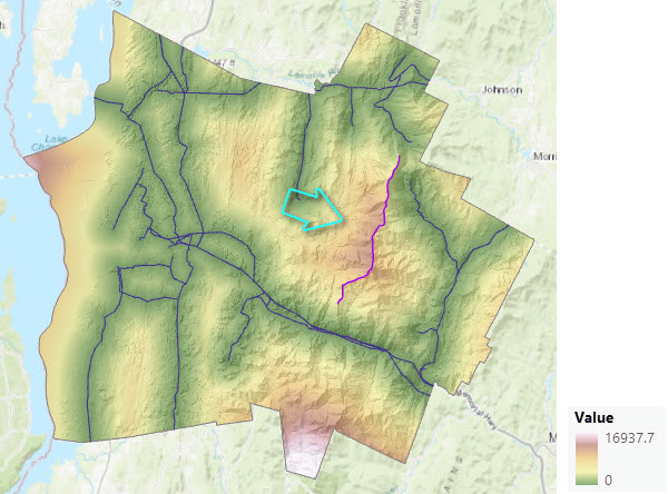
Because of local restrictions, new power lines cannot go over ridgetops. The following image shows the impact of adding a ridgeline (purple line) as a barrier. Note the locations on the other side of the ridge line are now farther (in light brown) from the power lines because of the added distance necessary to move around the ridge line.
Note:
If a barrier causes any locations to be disconnected from a source, no distance is calculated to the disconnected cells.
Back-direction and source-direction rasters
Distance accumulation also allows you to create a back-direction raster and a source-direction raster. For each nonsource cell, the back-direction raster identifies the direction that you travel when leaving the nonsource cell to return to the closest or least-cost source.
For each nonsource cell, the source-direction raster identifies the direction to the closest or least-cost source cell. If there are no barriers when calculating straight-line distance, these two outputs are the same; with barriers they are not.
The back-direction and source-direction rasters use the same convention as a compass. The range of values is from 0 degrees to 360 degrees, with 0 reserved for the source cells. Due east, to the right, is 90, and the values increase clockwise, so that 180 is south, 270 is west, and 360 is north. The two rasters report actual direction, with the back-direction raster reporting the degrees as floating-point values and the source-direction raster reporting them as integers.
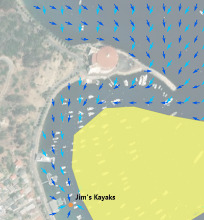
The difference between the back direction and source direction output is illustrated, for example, when calculating travel distance for a kayaker to reach a destination (Jim’s kayak rental) when a peninsula of land is between the kayaker and the destination. The peninsula becomes a barrier to the kayaker (traveler). In the image below, in the back-direction raster, each cell stores the direction the kayaker should move out of the cell to paddle back to Jim’s kayak rental since the kayaker must navigate around the land. This directional movement is indicated for representative cells by the dark blue arrows. In the source-direction raster, each cell stores the straight-line direction back to the Jim's kayak rental. This direction is indicated by the light blue arrows. The two directions are different. The dark blue arrows guide the kayaker around the peninsula, while the light blue arrows indicate the straight-line direction back to Jim’s kayak rental from any location regardless of the peninsula.
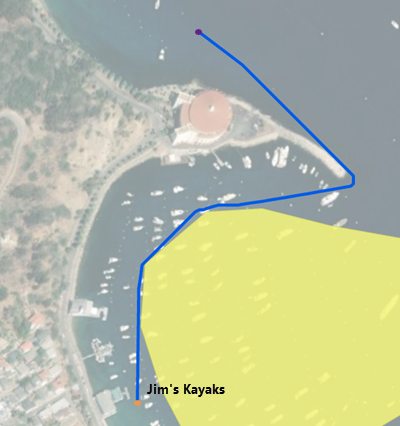
An important use of the back-direction raster is to generate shortest paths from a destination back to its closest source. In the image below, the output back-direction raster was an input to the Optimal Path As Line tool to define the shortest path the kayaker (purple dot) should take around the peninsula (the barrier), avoiding the boat moorings (yellow polygon), to return back to the kayak rental area.
Barriers can change the closest or least-cost source
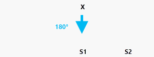
When barriers are added, they can change which source cell is the closest or least costly to reach. For example, in the first image below, there are two sources, S1 and S2. The closest source to nonsource cell x is source S1.
In the next image a horizontal barrier is added. The closest source to x is now source S2 (as shown by the light gray path around the right end of the barrier).
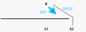
As a result, the presence of barriers can change the output values for cells in the back-direction raster. In this example, the value assigned to x in the back-direction raster without the barrier will be 180.0. With the barrier, the back direction for x will be 121.5.
For the source-direction raster, the closest source to cell x without the barrier is S1, south, at a direction of 180 degrees. When the horizontal barrier is added, the source direction assigned to x is approximately 135 degrees (light blue arrow), which is the straight-line direction from x to source S2, not the in-route direction. As a result of the barrier, the back direction and source direction from x to S2 are different.
The value for x in an output distance allocation raster will change from S1 without a barrier to S2 with the barrier.
If a cost surface and barrier are provided, the following three scenarios are possible for the value assigned to nonsource cell x:
- If S1 was the least-cost source without the barrier, with a barrier, S2 becomes the least-cost source with an accumulative cost greater than the value assigned to S1.
- If S2 was the least-cost source without the barrier, source S2 was initially cheaper to reach than S1. With a barrier, S2 is still the least-cost source to reach but the total accumulative cost is increased.
- S2 was the least-cost source without the barrier, but the path to reach S2 does not pass near the barrier. With the barrier, the accumulative cost for S2 remains the same. The barrier had no effect.
With a cost surface, the source-direction raster will change if the least-cost source for x changes from S1 to S2. However, if S2 was initially the least-cost source, the source direction for x will remain the same.
Thicken barriers to prevent cracks
A barrier can be represented as a linear feature, such as a road or river. In this case, the line feature must be rasterized before the distance operation is performed. As a raster, the linear feature will be only one cell thick. While the nature of the barrier would be preserved where it is perfectly horizontal or vertical, it may be diagonal. In this case, it is geometrically possible for the traveler to slip through what amounts to cracks in the barrier.
To prevent this, the Distance Accumulation and Distance Allocationtools automatically thicken the diagonal sections by one cell. Since the traveler is prevented from passing through the diagonals, the barrier input will remain a true barrier.

If the input barrier is a raster, this thickening process also occurs for the diagonal cells that are one cell wide.
Barriers that are specified as a dataset in the tool parameter are merged into the cost surface and, where necessary, NoData cells in the cost surface are thickened. As a result, the barriers are thickened regardless of whether they are specified by a dataset or their locations are assigned NoData in the cost surface, which avoids potential cracks.