Available with Image Server
The Optimal Region Connections tool identifies the optimal network of least-cost paths to connect a series of input regions. It does not create separate paths connecting one location to another.
Use this tool if you have a number of regions and want to create a network that plots how to travel between them in the best way. For example, the regions can be a series of habitat patches, parks, or logging operations. The resulting networks can be wildlife corridors connecting the habitat, bicycle trails connecting the parks, or logging roads connecting the logging operations.
In the resulting network, the traveler can move from one region to any other region using the paths, including traveling through other regions to reach a distant region.
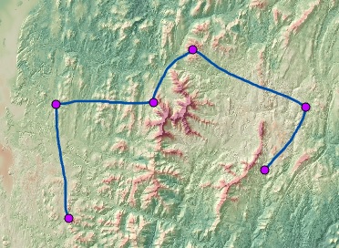
If you provide a cost surface input, the resulting network will be a network of least-cost paths. If you only provide input sources, the resulting network will be the network of the shortest paths.
In the optimal network, the direction of travel does not matter. The accumulative cost is the same whether the traveler moves from one region to another region or from the second region back to the first. If the direction of travel is relevant to your analysis, use the Optimal Path as Line tool.
Optimal network application examples
An optimal network of least-cost paths between locations can be used to solve various scenarios, such as the following:
- In a disaster relief effort, you have identified five areas where rescue and medical staff camps will be positioned. You want to develop the best network of supply routes between the camps.
- In a timber harvest, you want to create the most cost-efficient network of logging roads from which to extract the lumber.
- In a firefighting operation, you want to identify the best network of trails to move firefighting resources between various headquarters.
- From a suitability model, you have identified 10 of the best habitat patches for bobcat. You want the bobcats to be able to move between the patches through the most effective network of wildlife corridors to maintain genetic diversity within the metapopulation.
Optimal network analysis
Distance analysis can be divided conceptually into the following related functional areas:
- Calculate straight-line distance and optionally adjust the calculations with a barrier or surface raster.
- Optionally determine the rate the distance will be encountered using a cost surface, source characteristics, vertical factor, and horizontal factor. Create the accumulative distance raster.
- Connect regions over the resulting accumulative distance surface using an optimal network, specific paths, or corridors.
From the third functional area, connecting regions with an optimal network of paths is illustrated below. The scenario involves a collection of four regions that correspond to forest ranger stations (purple dots), and some rivers (blue lines).
The regions are connected by an optimal network over the cost surface while applying a barrier.
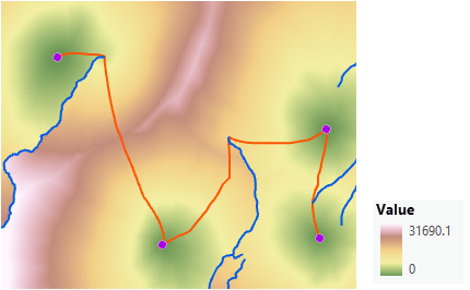
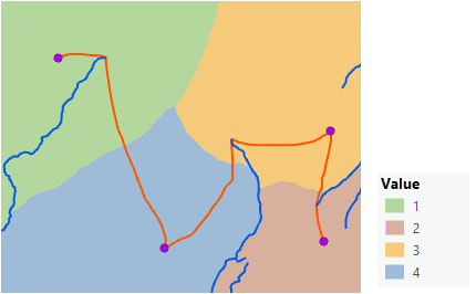
By examining the distance allocation output, it can be seen why the two lower regions are not connected. Due to the river barrier they are not cost neighbors.
Create an optimal network
To create an optimal network output, complete the following steps:
- Open the Optimal Region Connections tool.
- Provide the regions to connect in the Input raster or feature region data parameter.
- Name the output optimal connectivity network.
- Optionally, provide a barrier dataset.
- Provide a cost surface for the Input cost raster parameter if applicable.
- Optionally, provide a name for the Output feature class of neighboring connections parameter.
- Optionally, specify the Distance method or Connections within region parameter values.
- Click Run.
Optimal Region Connections tool
The Optimal Region Connections tool identifies the optimal network of least-cost paths to connect a series of input regions.
Provide the inputs
First, identify the source regions.
A region can be a point, line, polygon, or groups of raster cells. The regions identify the locations to be connected. The locations in a feature dataset are considered the regions. When the input is a raster, a region is a group of contiguous cells with the same value.
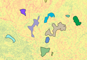
In the image below, the input regions (the colored polygons) are displayed over a cost surface layer.
Determine the least-cost region
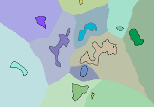
The least-cost region is identified for each nonsource cell using the calculations performed by the Distance Allocation tool.
In the image below, the input regions are displayed over the associated distance allocation layer. The value of each cell in the allocation raster identifies the region that can be reached with the cheapest (lowest) accumulated cost.
Create cost paths
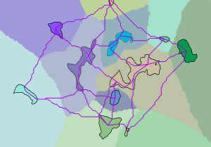
Cost paths are created between each region and its neighboring cost regions.
In the image below, the input regions and the least-cost paths from each region to its neighboring cost regions (magenta lines) are displayed over the associated cost allocation layer.
Convert regions and paths to a graph
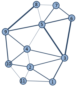
The regions and the resulting paths are converted to a graph. A graph in this context is the mathematical structure used to model pairwise relationships through graph theory. In the conversion, the regions are the vertices and the paths are the edges. The accumulative cost for the path is the weight for the edge.
Conceptually, this conversion is represented by the following illustration. The numbered circles are the vertices (the regions) and the connecting lines between the vertices are the edges (the least-cost paths). The weights for the edges are the accumulative cost for the paths. In the illustration, higher costs are represented by thicker lines.
Note:
To fully understand how this tool works, it is recommended that you have a basic understanding of graph theory. Many resources are available for this, but you can start with the Wikipedia entry at https://en.wikipedia.org/wiki/Graph_theory.
The minimum spanning tree is determined using graph theory to connect the vertices (regions) in the most effective (least cost) way. The minimum spanning tree is not necessarily unique since there may be more than one set of edges that are deemed best.
Note:
More information about minimum spanning trees is available online, such as the Wikipedia entry at https://en.wikipedia.org/wiki/Minimum_spanning_tree.
Map to line features
The spatial representation of the regions and the paths from the minimum spanning tree are mapped back to an output feature class.
In the image below, the input regions and the least-cost path network from the minimum spanning tree (magenta lines) are displayed over the associated cost surface layer.

Output paths to neighboring cost regions
Optionally, a feature class of the paths to the neighboring cost regions can be output. You can use this output to create your own network, add paths to your minimum spanning tree, or further analyze it in network analysis.

If no cost surface is provided, the output would be a network of paths that connects the regions the shortest way possible.
Note:
The Optimal Region Connections tool honors barriers. Barriers can be specified by the barrier parameter or by NoData cells in the mask or in the cost surface raster. The resulting network identifies the shortest or least costly physical distance to reach each location from a source while navigating around these barriers.
Additional information
The following sections contain additional information regarding connecting regions with an optimal network of paths.
Paths continuing through regions
Each path is a separate linear feature and duplicate lines will exist where the paths travel a common segment.
For a connected network of paths, if the input regions are polygons or a raster of multicell regions, the paths are continued to a point within the region to allow the traveler to enter by one path, move within the region, and exit by another path to reach other regions. Since it is unknown how a traveler will move within the region, no cost is assigned to these extended segments within a region and no cost is incurred when moving through the region. The same is the case when linear regions are input: no cost is incurred when moving along the linear region to reach other paths.
To illustrate the resulting connected network relative to a series of independent least-cost paths, the image below shows the difference between the two ways regions can be connected. The first image shows the result of using the output from the Distance Accumulation tool as input to the Optimal Path As Line tool. In this case, the paths only reach the edges of the regions. The second image shows the resulting network of paths connecting the regions created by the Optimal Region Connections tool. In this result, the paths continue within the region, allowing the traveler to enter the region by one path and leave by another.

Since the output from Optimal Region Connections is a topologically correct network, it can be used in network analysis to perform additional analysis.
You can also use the Optimal Region Connections tool to prevent paths from continuing through the regions by specifying No connections for the Connections within regions parameter.
Optimal Region Connections and Optimal Path As Line tools
The Optimal Region Connections tool creates an optimal network of paths between a number of input regions. The Distance Accumulation and Optimal Path As Line tools work in combination to create paths between identified sources and destinations. The Distance Accumulation and Optimal Path As Line tool sequence can also be used to create a network of paths by iteratively isolating a region as a source and connecting it to the other regions identified as destinations. This process is repeated for each region and the resulting least-cost paths are combined.
The following are limitations to the iterative approach:
- Connecting each region to all other regions is a combinatorial process that can create a very large number of paths, especially when there are a lot of regions. This approach does not allow a distant region to be reached by using a series of paths connecting a sequence of regions that are between you and the distant region.
- To reduce the potential for large numbers of paths, many times the closest straight-line distance between two regions is used to identify the source and the destination. However, while two regions can be close together geographically, it may be costly to travel between them because of an intervening feature such as a mountain or a river. The Optimal Region Connections tool determines the regions to connect based on least-cost proximity.
- Many times, different paths from different regions join and follow the same least-cost path to a common region. It is difficult to analyze the shared portion if they are raster paths, such as those created by the Optimal Path As Raster tool. When performing subsequent analysis, it is better if each path is treated as a separate entity.
- Paths created by the Optimal Path As Line tool only reach the edge of a region. They do not create a connected network of paths.
Regions and zones
Regions are used as the input to Optimal Region Connections. The regions can be either a feature or a raster dataset. If the input regions are feature data, the features are converted to a raster. A region is any group of contiguous cells with the same cell value. A zone is all cells of a raster that have the same value. Zones can be composed of a single region or multiple disconnected regions. For Optimal Region Connections, if there are groups of cells in the input with the same value that are not connected to each other, they are treated as a single region with disconnected cells. The result is that only the group of cells within the region that is the least costly to reach will be connected in the network, so not all of the cells in the input will be connected.
An input that contains multiple disconnected groups of cells can be converted to a series of independent regions using the Region Group tool. Using the output from Region Group as input to Optimal Region Connections will connect each region to all other regions, so all cells in the input can be reached through the resulting network.
Sample scenarios using the Optimal Region Connections tool
The following are common scenarios for using the Optimal Region Connections tool.
- The optimal network (the minimum spanning tree) is the desired output.
- Add specific paths to the optimal network using Distance Accumulation and Optimal Path As Line to connect regions that the optimal network did not capture. For example, when fighting multiple forest fires, add escape routes for firefighters to use if conditions change.
- Create the network from the optional output of all paths to the neighboring regions. Use the Select tool to select the paths.
- Turn any of the above scenarios into a network and perform additional analysis of the movement between the regions.