Available with Image Server
The objective of creating optimal paths is to connect specific sources with specific destinations.
In contrast, the Optimal Region Connections tool connects a series of input regions with the optimal network of paths. Which regions are connected to which is determined by the least-cost calculations. The direction of travel between the regions does not matter. This means that traveling from region A to region B has the same accumulative distance as traveling from B to A.
If you want a specific location to be connected to another specific location, or the direction of travel between the locations matters, use the Optimal Path as Line or Optimal Path as Raster tool.
When the direction of travel matters is evident when going uphill or downhill between two locations. It takes more effort to move uphill and it takes longer to cover each distance unit. Moving downhill takes less effort and the traveler can cover each distance unit at a faster rate. This effort is referred to as a vertical factor. Direction also matters when a horizontal factor is present, such as moving with or into the wind. Moving with a tail wind requires less effort than traveling into a headwind.
To connect specific locations with optimal paths, you'll do the following:
- Use the Distance Accumulation tool to calculate the accumulative distance and back-direction rasters from the input sources.
- Use either the Optimal Path As Line or the Optimal Path As Raster tool to create the optimal paths. Provide the destinations and the distance accumulation and back-direction rasters created above.
If any rate controlling factors, such as cost surface, source characteristics, vertical factor, and horizontal factor, were entered into the Distance Accumulation tool, the resulting path will be the least-cost path. If no rate controlling factors were entered, the resulting path will be the shortest path between the two locations.
Optimal path application examples
Connecting locations with the optimal path can be used to solve various scenarios, such as the following:
- Find the shortest water distance from one port to another, staying within 2 miles from the coast where possible.
- Identify the optimal path between two wildlife patches so that you can determine the properties you need to acquire to allow the animals to move between the patches.
- Establish a network of trails for firefighters to use to move between a series of ongoing wildfires. Due to the severity of one of the fires, even though there is one primary trail to the fire, you want to add a second trail that can be used as an escape route.
- In a logging operation, identify the cheapest route for a logging road that can be used to extract logs.
- Identify the straight-line flight path for a crop duster to reach a field that must be sprayed.
Optimal path analysis
Distance analysis can be divided conceptually into the following related functional areas:
- Calculate straight-line distance and optionally adjust the calculations with a barrier or surface raster.
- Optionally determine the rate the distance will be encountered using a cost surface, source characteristics, vertical factor, and horizontal factor. Create the accumulative distance raster.
- Connect regions over the resulting accumulative distance surface using an optimal network, specific paths, or corridors.
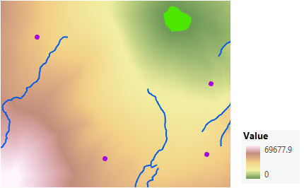
From the third functional area, connecting locations with specific optimal paths is illustrated below. The scenario involves a collection of four forest ranger stations (purple dots), and some rivers (blue lines).
A new park is created (the light green polygon). It will be added to the ranger station least-cost network.
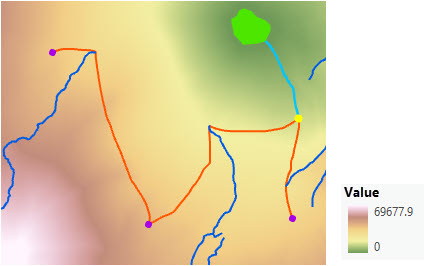
A path needs to be created from the park to the ranger station just south east of the park. The ranger station (the destination), the output accumulative distance, and the back-direction raster created in the Distance Accumulation tool are entered into the Optimal Path As Line tool.
Create an optimal path
It takes two short workflows to create an optimal path between locations.
Create the input distance rasters
First, create distance accumulation and back-direction rasters.
- Open the Distance Accumulation tool.
- Provide the source to connect to for the Input raster or feature source data parameter.
- Provide a name for the Output distance accumulation raster parameter.
- For straight-line distance, you can provide barriers and a surface raster. To consider the least-cost path, some or all of the rate controlling parameters, a cost surface, source characteristic, vertical factor, and horizontal factor, can also be provided.
- Provide a name for the Out back direction raster parameter.
- Click Run.
Determine the path
Then determine the optimal path:
- Open the Optimal Path As Line or Optimal Path As Raster tool.
- Identify the destination to connect from in the Input raster or feature destination data parameter.
- Identify the just created output distance accumulation raster in the Input distance accumulation raster parameter.
- Identify the just created output back-direction raster in the Input back direction or flow direction raster parameter.
- Provide a name for the Output optimal path as feature value.
- Select a value for Path type.
- Click Run.
Connect specific sources with specific destinations using optimal paths
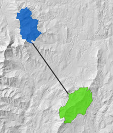
The objective of creating optimal paths is to connect specific sources with specific destinations. To identify the shortest straight-line path between the sources and destinations, you only need to identify the sources and destinations. The result is the path a low flying bird would take to move between the two locations.
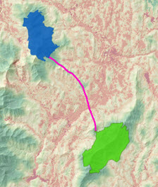
When a cost surface is entered, the output is a least-cost path. A least-cost path analysis finds the cheapest way to travel between the different locations. Given a set of sources, a set of destinations, and information on the difficulty of moving across the landscape captured in a cost surface, the least-cost paths are the cheapest way of connecting the locations. This simulates a traveler as they move through the landscape.
Optimal paths creation process
To create the shortest or least-cost paths between specific locations, two tools are used in sequence, Distance Accumulation and Optimal Path As Line (or Optimal Path As Raster). The workflow for creating the least-cost path is illustrated below using multiple destinations.
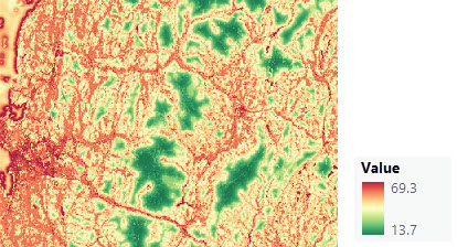
The input necessary for the analysis are the sources, a cost surface raster indicating the difficulty of moving through each cell, and the destinations. The result of the analysis is the least-cost path that connects the identified locations.
Tip:
Identifying the shortest paths between the locations follows the same workflow, except no cost surface is used.
Prepare input data
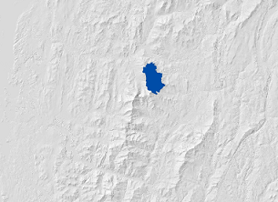
In the image below, the source input raster is the blue cells. This input is displayed on top of a hillshade of elevation raster background.
The cost surface input raster is shown below. The green areas represent cells with lower values, which indicate locations that are less costly and easier to move though. The color transition from green to yellow to red represents increasing cost.
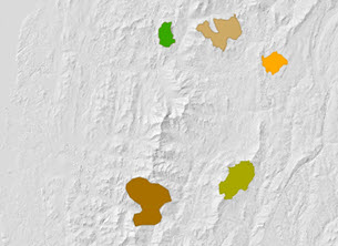
The destination input raster is shown below. Note that there are multiple destinations. This input is displayed on top of a hillshade of elevation raster background.
Create the accumulation and direction outputs
Run the Distance Accumulation tool with the source and cost surface inputs.
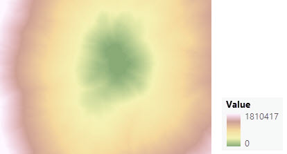
The output distance accumulation raster is shown below.
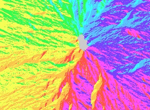
The output back direction raster is shown below. The color indicates the direction of travel when leaving a cell to move back to the cheapest source cell.
Create the path output
Run the Optimal Path As Line or the Optimal Path As Raster tool with the destinations you want to connect and the accumulative distance and back direction rasters created above.
Since there are multiple destinations, there are three options to determine how to connect the destinations to the source:
- Best single—Identify the shortest or least-cost path from the closet or cheapest destination.
- Each zone—Identify the shortest or least-cost paths from each destination back to the closest or cheapest source.
- Each cell—Identify the shortest or least-cost paths from each cell in the destinations back to the closest or cheapest source.
An example of the result from the Best single option is shown below.
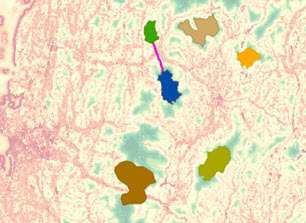
If the input locations are features, they are internally converted to a raster. The input can be groups of contiguous raster cells. The created paths connect the closest or cheapest cell in the destination to the closest or cheapest cell in the source.
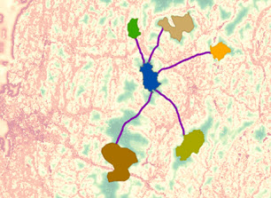
See the Additional information section below for more information regarding the Each cell option.
Account for path direction
You can explicitly account for the direction of travel between sources and destinations. In the optimal paths creation process, when using the Distance Accumulation tool you can incorporate directionality in the following ways:
- Use the Travel Direction source characteristic to specify whether the distance accumulation will be calculated moving toward or away from the sources.
- Account for the effort to overcome the encountered slopes with the vertical factor.
- Account for the effort gained or lost when encountering a horizontal factor, such as wind or current.
By itself, the Travel Direction parameter has no effect on the calculations and the resulting path. However, when combined with vertical and horizontal factors, which are dependent on the direction the traveler is moving, the resulting paths will vary.
The vertical factor accounts for the effort expended to overcome the encountered slopes when moving toward or away from a source. If the mover is going uphill, it takes more effort and time to travel each distance unit. If going downhill, the distance can be covered at a faster rate. If moving with the contours, slope is essentially flat. For additional information about applying a vertical factor, see Adjust the encountered distance using a vertical factor.
As with the vertical factor, the horizontal factor is influenced by the direction the traveler moves through a cell. A boat heading into a strong wind or current imposes a resistance that the traveler must overcome, so the distance units are covered at a slower rate. Moving with the wind or a current, the boat may cover the distance at a faster rate. As a result, the angle the wind or current is encountered when moving into a cell matters. For additional information about applying a horizontal factor, see Adjust the encountered distance using a horizontal factor.
Moving away from a source or toward a source will alter how the traveler moves through the cell, changing how they encounter the vertical and horizontal factors in that cell.
Example: Route a powerline
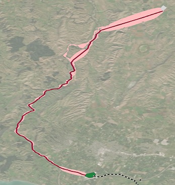
You want to determine an optimal path for a new powerline. The path may be impacted by several factors, such as the cost to acquire land and build on it, regulations keeping the path away from inhabited areas, and by the potential for being excessively visible. In addition, a path that follows level ground will be easier to build on than one that is frequently going uphill and downhill.
These factors, along with a set of proposed starting points (sources) for the powerline path, are used as inputs to the Distance Accumulation tool. The land acquisition and building costs and visibility potential are weighted and combined into a cost surface. The same costs will apply regardless of direction of travel through a cell.
A regulatory buffer around towns is used for the barriers parameter. A horizontal raster and associated factor can be used to encourage routes that follow contour lines and avoid moving uphill or downhill. In this case, the direction of travel between the sources and destinations is not important (the horizontal factor function will be symmetric). The Distance Accumulation tool creates the accumulative distance and back-direction rasters.
Then use either the Optimal Path As Line or the Optimal Path As Raster tool. The accumulative distance and back-direction rasters, along with the proposed destinations are input. The output from Optimal Path As Line is a polyline feature class delineating one or more paths that connect destinations and sources in an optimal way. The output from Optimal Path As Raster is a raster that represents the intensity of usage, or popularity, of a cell as measured by the number of routes passing through it. It is analogous to how the flow accumulation raster is created by tracing through a flow direction raster.
Least-cost path analysis
To have confidence in the resulting paths consider the following:
- Can the input data answer the questions that you are asking?
- Is the raster resolution appropriate?
- Are the units of the cost surface correct?
- Did you account for directionality?
- In the cost surface, how were the values in a criterion transformed and the weights between criteria determined?
- Is there a way to test your results to see if they make sense?
Resolution of the input data
You can use least-cost path analysis to determine 1- and 2-hour search radii for a missing person. If you use a 30-meter land cover raster as one of your criteria, your cost path analysis may not identify the types of paths that a search and rescue team can use when travelling on foot. Also, at this resolution, the paths may ignore real barriers. In both cases, the resulting paths may allow travel options that do not exist in the terrain. On the other hand, a 30-meter elevation raster may be sufficient as the vertical factor raster to weight the per-cell cost in the travel direction.
Distance accumulation input units
The Distance Accumulation tool multiplies the rate in the input cost surface (which may be implicitly 1) by the cell size, which is expressed in linear units. It is important that you do a dimensional analysis of the cost surface to verify that the output accumulative cost raster has the expected units (such as travel time, dollars, or energy). See the Distance accumulation algorithm topic for more information about units in distance analysis.
Verify the results
In the powerline example above, you should determine how good the proposed path is. One way to do this is to use the same data and modelling workflow to predict the as-built location of an existing powerline. If they differ, can you explain the difference?
Additional information
The following sections provide additional information regarding connecting locations with optimal paths.
Convergence of multiple paths
The Optimal Path As Line tool outputs a feature class containing one polyline per destination. Each polyline has an attribute that provides the total accumulation cost to move between the destination and the source. Another attribute provides the identity of the destination. If multiple paths converge and travel the same route back to the source, there will be multiple lines on top of each another, one from each destination. Optimal Path As Line is the more commonly used tool when identifying the least-cost paths.
The Optimal Path As Raster tool outputs a raster that identifies the least-cost path (one cell wide) to use to move between the destination and the source. The output cell values in the paths indicate the number of paths from the destinations that pass through that cell. When there is one destination or multiple destinations and the paths do not overlap, all cells along the paths will contain the same value.
If there are multiple destinations and the paths converge, each cell will record the number of paths that pass through that cell.
The output from Optimal Path As Raster indicates the intensity of use. When identifying wildlife corridors from multiple habitat patches, for example, the cells with the higher values along the paths indicate that the segment of the paths is the most critical because many of the paths rely on it. If certain segments are used by many paths, you may want to protect those segments first.
Least-cost path creation
In the powerline example above, the Distance Accumulation tool created a distance accumulation and a back-direction raster. The distance accumulation raster has cell values in units of dollars and expresses the total construction cost to reach each cell from a source cell. The back-direction raster provides travel directions from each cell back to its cheapest source. The travel direction is expressed as a map azimuth (clockwise from grid north) in the range of 0 to 360, in which zero is reserved for source cells.
The Optimal Path As Line tool uses both of these datasets to plot least-cost paths starting from a set of destination locations. The destinations can be either a feature class or a raster dataset. If a feature class is used, it is first rasterized and the cell centers containing data values are used as the destinations. The analysis is always done in the spatial reference, extent, and cell size of the back-direction raster.
The path is created by tracing the back-direction raster from the destination to the source. Starting from the cheapest cell in the destination, the back-direction raster identifies the next cell to move into to produce the least-cost path back to the source. Then the value of that cell, obtained from the back-direction raster, identifies the next cell to move into. This process continues until the source is reached.
By default, each output polyline defines a complete path from a destination back to its cheapest source. The feature class includes fields for the ID of each input destination, its accumulative cost, and its starting row and column.
If the Create network paths parameter is checked in the Optimal Path As Line tool, the schema of the output polyline feature class changes. Each feature will describe an edge in a network that connects destinations to sources. Each edge has an EdgeCost attribute that provides the change in accumulative cost as you travel along the edge. See the Use Optimal Path As Line to create least-cost path networks section below for more information.
Note:
The optimal paths are not forced to pass through the cell centers en route from the destination to the source. When determining the accumulative cost for each cell, a plane is fit. The direction of the gradient of the plane determines the true direction to leave that cell en route to the shortest or cheapest source. From the back direction, the path is adjusted using a lattice structure to create the resulting path. The path travels a more direct direction through the cells, creating a more accurate result. For details of how the distance accumulation and the paths are calculated see Distance accumulation algorithm.
Optimal path tools with flow accumulation and flow direction rasters
For the Optimal Path As Line and Optimal Path As Raster tools, the input to the accumulative distance raster parameter can be the output from the Flow Accumulation tool, and the input to the back direction raster parameter can be the output from the Flow Direction tool. In this case, these tools will trace stream routes until they either flow off the edge of the dataset or stop on a cell of undefined flow. The Create network paths parameter is useful in this case because it generates a stream network that can be used with one of the Esri network solutions. The stream edges are oriented in the flow direction and the EdgeCost attribute is the change in flow accumulation over the length of the edge.
Impact of altering the path type and configuration of the destinations
In the powerline example above, the accumulative cost and back-direction rasters were constructed from a single source cell representing one end of the proposed powerline, for example, an existing substation. By exploring different path types and configurations of input destinations with the Optimal Path As Line tool, you can examine how the least-cost paths can change and the impact that will have. The following are common scenarios:
- There is a known destination as a single point. You want to find the best path between that destination and a source that is also a point. In this case, it doesn’t matter which path type is selected. The Optimal Path As Line tool will find the best path between the two locations and produce a single feature in the output polyline feature class.
- There are a set of distinct candidate destination points and you want to compare the paths from each. Select either Each zone or Each cell for the path type, since each destination is a different zone.
- There is a single, multicell contiguous region destination, and you want to determine the location within the region with the least construction cost and the path from that location to the source. Select either the Best single or Each zone path type. If there are multiple contiguous regions, specify Each zone to compare the best paths from each.
When there are many destinations, the paths may merge as they move toward a source. A least-cost path can be considered the steepest downhill path on an accumulative cost surface.
Merging paths can be used to analyze the movement of students in a community to a school. Optimal Path As Raster indicates how paths pass through a cell or how popular a cell is. Using the Each cell path type and a multicell destination as the input to the tool, you can determine which cells are used more by students as they travel from locations within a study area to the school.
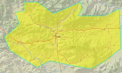
The output shows the intensity of cell usage as students travel from every cell in the study area to the school. This is essentially a "flow accumulation" map of student travel, instead of water travel. This intensity information can be used to help decide where improving street safety affects the most students (assuming students are distributed evenly in the study area)
Use Optimal Path As Line to create least-cost path networks
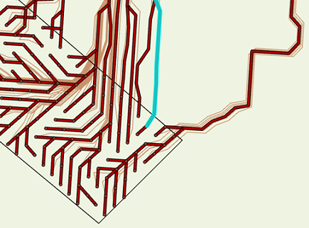
By default, the output of Optimal Path As Line creates a separate feature for each path traced from a destination to a source. This can introduce many overlapping or nearly overlapping polylines into the output. You can use Optimal Path As Line to create nonoverlapping polyline feature classes that can be used as an input to one of the Esri network solutions, as a network dataset, utility network, or trace network. When you check the Create network paths parameter, multiple paths that enter a single cell are snapped to that cell center and are terminated. The multiple paths are merged as a single path to create a network. A new path uses that cell center as its starting location. Also, the schema of the output polyline feature class changes. The EdgeCost attribute reports the change in accumulative cost along the edge, instead of along the complete path.
This works with flow direction input as well as back-direction conventions. When flow direction is used, the input accumulation raster must be a flow accumulation raster.
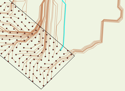
Many paths will converge into a single path when the Create network paths parameter is checked.
Identify alternative starting locations for least-cost paths
In the powerline example, it was known that the powerline was to end at the substation. But if a polygon, such as a parcel, was entered as the destination using the Best single path type, only one starting point within the destination would be identified.
With a polygon destination, there is one cheapest path to reach it, but there are many other possible alternatives to enter the polygon. As a result, the goals of the analysis change to the following:
- Determine the flexibility for creating a path from a single destination to a destination that has multiple cells.
- Identify the paths that are close in cost that are possible alternative solutions. That is, for multiple destinations, the cost from destination A may be 1 and the cost from destination B may be 1.0001. Best single will only identify the least-cost path and you won't know if there are viable alternative paths.
- Identify the possible path options given a specified cost threshold.
- Determine the flexibility of a source location. That is, start with a multicell source and see how the cost paths are distributed around it.
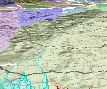
If the Each cell path type is applied, other possible starting points within the destination can be explored. In the image below, all the potential paths (brown lines) are calculated from each cell in the destination back to the source. The highlighted paths are roughly the top 10 percent of the cheapest paths from all the potential paths. They share substantially the same route back to the source, and they will have similar cost. Choosing a path that is similar in cost to the least-cost path may provide flexibility in determining which destination cell location to start the path from to reach the source.
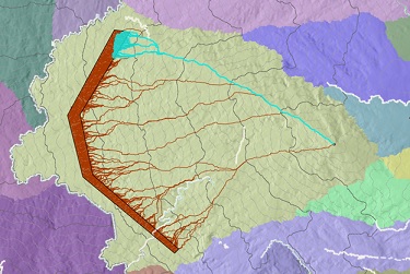
This becomes more obvious in a 3D view in which you can see that this group of paths are all located in a subwatershed of the accumulative-distance raster.
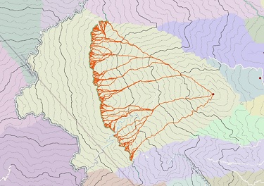
For the third analysis goal, you may have a strict fixed cost for your path and want to see the possible alternatives. In this case, notice that all locations on a contour line of your accumulative-distance raster (the contour lines are identified in the image below) have the same cost. A path starting from any point on that contour will have the same cost.
You can use the Con tool to identify the destinations that have the same cost. For example, select a travel time contour from the accumulative cost raster SchoolTravelTime with the following expression:
equalCostPathDestinations = Con((Raster('SchoolTravelTime') > 19.9) & (Raster('SchoolTravelTime') < 20), 1)The resulting set of raster cells in the destination show that the resulting distribution of paths all have the same cost and travel time to the same source, meeting the fixed cost limit.
For the fourth analysis goal, the paths start at the same destination, have roughly the same cost, but they are traveling to separate sources. In the image below, multiple sources were entered.
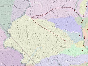
The paths travel to source locations in different areas, which indicates that they are on or near an allocation boundary. This is an unstable situation because the boundary could shift depending on uncertainty in any of the inputs to Distance Accumulation. This uncertainty could slightly alter the accumulative cost, potentially changing the source one of the paths would travel to. Using the above flow analogy, if you are standing on the ridgeline of a watershed, a small step away from the ridge can have a big impact on which way you continue downhill.
Least-cost corridors
You can use least-cost corridors to visualize a set of least-cost paths all at once. You can also use them to visualize the sensitivity of an almost least-cost path to changes in its cost. For additional information, see Connect regions with corridors.